In practice, we regularly use the linear, tree, or ensemble models but we are also seeing use cases of Generalized Linear Models (GLMs) and Generalized Additive Models (GAMs). As a matter of fact, both linear regression and logistic regression are special cases of GLM with Gaussian distributions and Bernoulli distributions, respectively. Today’s focus would be on the TweedieRegressor from sklearn which is a Generalized Linear Model with a Tweedie distribution. However, before we move on, let’s understand these terms.

What is the Generalized Linear Model?

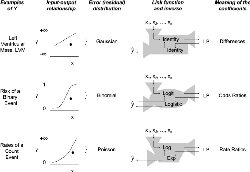
Generalized Linear Models or GLMs can be of both regression and classification types but the main parameter considered in both cases is the type of distribution the data follows. GLM models allow us to build linear relationships between responses and predictors, despite their underlying nonlinearity. In order to accomplish this, a link function is used, which connects the response variable to a linear model. There is no need to assume a normally distributed error distribution for the response variable in Linear Regression models. Response variables are assumed to follow an exponential distribution family (e.g. normal, binomial, Poisson, or gamma). The GLM consists of three elements:

1. A particular distribution for modelling from among those which are considered exponential families of probability distributions

2. A linear predictor

3. A link function.

What is Tweedie distribution?

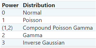
Tweedie distributions represent a family of probability distributions in probability and statistics. They consist of a continuous normal distribution, a continuous gamma distribution, an inverse Gaussian distribution, a discrete scaled Poisson distribution, and a compound Poisson–gamma distribution. The Tweedie distribution is a special case of an exponential distribution. It has three parameters mean(μ), variance(σ2), and shape(ρ). Based on the shape we can define what distribution the data is following as

• p = 0: Normal distribution,

• p = 1: Poisson distribution,

• 1 < p < 2: Compound Poisson/gamma distribution,

• p = 2 Gamma distribution,

• 2 < p < 3 Positive stable distributions,

• p = 3: Inverse Gamma distribution,

• p > 3: Positive stable distributions,

• p = ∞ Extreme stable distributions.

The distribution is not defined for values of p from 0 to 1.

TweedieRegressor

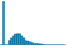
TweedieRegressor can handle semi-continuous data as well as data with non-negative right-skewed distributions. TweedieRegressor can be imported from the sklearn linear_model module. We define p as power instead of shape, which determines the underlying distribution. The default power(p) value is 0. The allowed values are 0,1,2,3 representing Normal, Poisson, Gamma, and Inverse Gaussian distributions respectively. Another important parameter is the link function. It accepts three values namely auto, identity, and log. Using the auto setting, the link function is set based on the power value, while using the identity setting for values less than 0 and the log setting for values greater than 0.

Basic sample code:

from sklearn.linear_model import TweedieRegressor
reg = TweedieRegressor()
X = [[1, 2], [2, 3], [3, 4], [4, 3]]
y = [2, 3.5, 5, 5.5]
reg.fit(X, y)

reg.score(X, y)
#output - 0.839

reg.predict([[1, 1], [3, 4]])
#output - array([2.500..., 4.599...])

TweedieRegressor vs LinearRegressor

The dataset used in this example is taken from https://data.princeton.edu/wws509/datasets/#ceb. You can download the data by running this command in the terminal:

wget https://data.princeton.edu/wws509/datasets/ceb.dat
# or if using colab use this
!wget https://data.princeton.edu/wws509/datasets/ceb.dat

1. Importing necessary libraries

import pandas as pd
import numpy as np
import matplotlib.pyplot as plt
from sklearn.linear_model import LinearRegression
from sklearn.linear_model import TweedieRegressor
from sklearn.model_selection import train_test_split as tts
from sklearn.metrics import
r2_score,mean_absolute_error,mean_squared_error
import warnings
warnings.filterwarnings('ignore')

2. Reading data and doing preprocessing of categorical variables

df = pd.read_table("/content/ceb.dat", sep="\s+")df.replace({'0-4':0,'5-9':1,'10-14':2,'15-19':3,'20-24':4,'25-29':5},inplace=True)
df.replace({'Suva':2,'urban':1,'rural':0},inplace=True)
df.replace({'none':0,'lower':1,'sec+':2,'upper':3},inplace=True)

3. Splitting train and test sets

x = df.iloc[:,:-1]
y = df.iloc[:,-1]
x_train,x_test,y_train,y_test =tts(x,y,test_size=0.25,
random_state=43)

4. Fitting LinearRegressor

lin_reg = LinearRegression()
lin_reg.fit(x_train,y_train)
y_pred = lin_reg.predict(x_test)print('R2:',r2_score(y_pred,y_test),'MAE:',mean_absolute_error(y_pred,y_test),'MSE:',mean_squared_error(y_pred,y_test))#output - R2: 0.9043807418278866 MAE: 53.618762296898325 MSE: 3459.763241349285

5. Fitting TweedieRegressor

tweedie_reg = TweedieRegressor(power=1)
tweedie_reg.fit(x_train,y_train)
y_pred = tweedie_reg.predict(x_test)print('R2:',r2_score(y_pred,y_test),'MAE:',mean_absolute_error(y_pred,y_test),'MSE:',mean_squared_error(y_pred,y_test))#output - R2: 0.9026853686659407 MAE: 29.21429903857763 MSE: 2610.661935003697

Conclusion

From the above example, it is quite clear that the r2 score is nearly identical but if we see the difference in mean absolute error then surely the TweedieRegressor outperforms LinearRegressor. Thus proving if the distribution is other than a normal distribution, trying out TweedieRegressor won’t be a bad choice.

Follow me on Linkedin for collaborations and discussions related to ML, DL, data science, and MLops.