

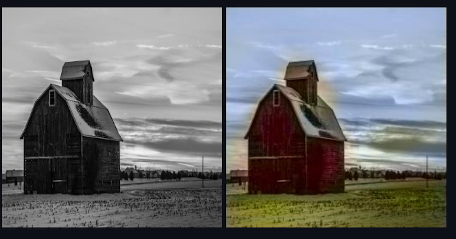


Image colorization is the process of assigning colors to a single-channel grayscale image to produce a 3-channel colored image output. Before moving to the code section, let’s understand what an AutoEncoder is!!!
What is an Autoencoder?
Autoencoders are a type of self-supervised learning model that can learn a compressed representation of input data. An autoencoder is a neural network model that seeks to learn a compressed representation of the input. They are an unsupervised learning method, although technically, they are trained using supervised learning methods, referred to as self-supervised. There are various types of autoencoders like Sparse autoencoders, Denoising autoencoders, Variational autoencoders, LSTM autoencoders etc.
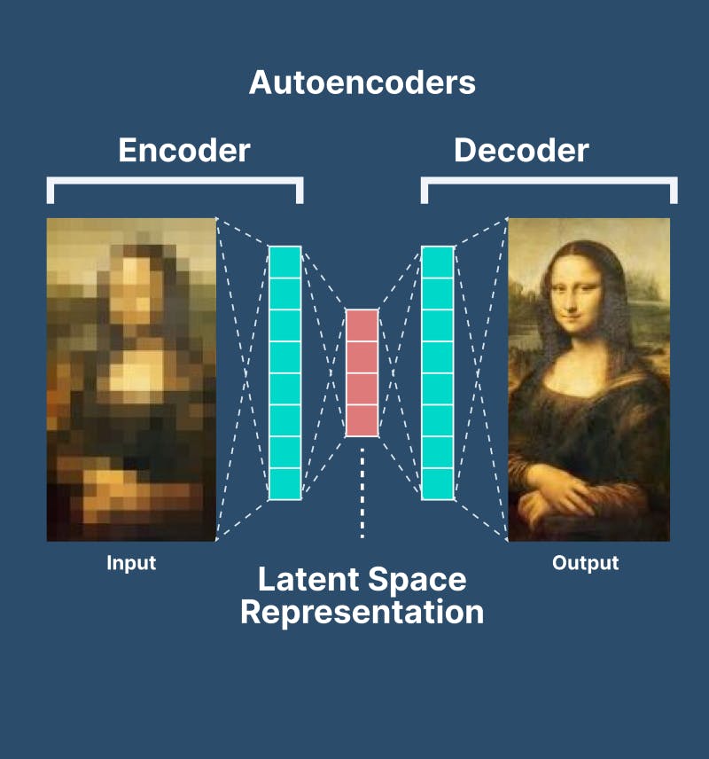
Source: V7 labs
Applications of autoencoders include:
Anomaly detection
Data denoising (ex. images, audio)
Image inpainting
Information retrieval
Dataset Information
Here for this example, I have taken a custom image dataset of a barn. Initially, I downloaded 12 images from google but that was not yielding much accuracy so I used the image augmentation technique to produce 84 images from those 12 images. The sample code for augmentation:
from tensorflow.keras.preprocessing.image import array_to_img,img_to_array,ImageDataGenerator,load_img
datagen = ImageDataGenerator(rotation_range=40, width_shift_range=0.2,height_shift_range=0.2, shear_range=0.2, zoom_range=0.2,fill_mode='nearest',horizontal_flip=True,)
img = load_img('photo')
x = img_to_array(img)
x = x.reshape((1,)+x.shape)
i=0
for batch in datagen.flow(x,batch_size=1,save_to_dir='path',save_prefix='1',save_format='jpeg'):
    i+=1
    if i>5:
        break
Link to the dataset images folder created by me.
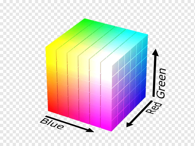
Color Models (RGB and LAB)
The RGB color model is one of the most widely used color representation methods in computer graphics. It uses a color coordinate system with three primary colors: Red, Green, and Blue. Each primary color can take an intensity value ranging from 0(lowest) to 1(highest). Mixing these three primary colors at different intensity levels produces a variety of colors. This is the basic color model which is used in most of the colour image processing problems while grayscale images are used for B/W processing tasks.
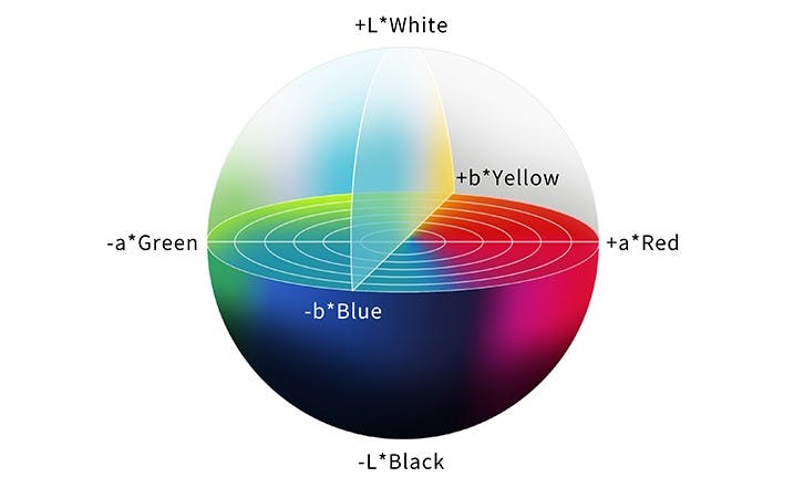
Another color model that will be actually helpful in our project is the LAB color model. Using this model we are going to train our Autoencoder. In LAB or CIE L*a*b*, L* axis represents Lightness, ranging from 0–100. 0 is black (no light); and 100 is white (maximum illumination). The a* axis is green at one extremity (represented by -a), and red opposite it at the other (+a). The b* axis has blue at one end (-b), and yellow (+b) opposite it at the other. In theory, there are no maximum values of a** and b**, but in practice, they are usually numbered from -128 to +127 (256 levels). This color model is extensively used in many industries apart from printing and photography.
Autoencoder Model
Let's start by importing all the required libraries and reading the images through ImageDataGenerator from TensorFlow. Since the L channel encodes only the intensity, we can use the L channel as our grayscale input to the network. From there the network must learn to predict the a and b channels. Given the input L channel and the predicted ab channels, we can then form our final output image. After that, we would split our images into X and Y where X represents L and Y represents A and B from the LAB color model. Please note that after converting X into L space it will only have the shape (32,256,256) so we have to reshape it into the (32,256,256,1) by adding 1 to its original shape to show that it is a single channel grayscale image.
import numpy as np
import tensorflow as tf
import matplotlib.pyplot as plt
from tensorflow.keras.layers import Conv2D, UpSampling2D
from tensorflow.keras.models import Sequential
from tensorflow.keras.preprocessing.image import ImageDataGenerator, img_to_array, load_img
from skimage.color import rgb2lab, lab2rgb
from skimage.transform import resize
from skimage.io import imsave,imshow

train_datagen = ImageDataGenerator(rescale=1. / 255)
train = train_datagen.flow_from_directory('path',target_size=(256, 256),class_mode=None)

X =[]
Y =[]
for img in train[0]:
      lab = rgb2lab(img)
      X.append(lab[:,:,0])
      Y.append(lab[:,:,1:] / 128)

X = np.array(X)
Y = np.array(Y)
print(X.shape)
print(Y.shape)

X = X.reshape(X.shape+(1,))
print(X.shape)
print(Y.shape)
Encoder-Decoder Architecture:
The encoder encodes/compresses and finds patterns/important features from the images to learn while the decoder decodes the compressed image to its original version to predict the output. We will be using the functional model API instead of using sequential model API. The code for the encoder and decoder are as follows:
class Encoder(tf.keras.Model):

  def __init__(self):
    super(Encoder,self).__init__(name='Encoder')
    self.conv1 = Conv2D(64, (3, 3), activation='relu', padding='same', strides=2, input_shape=(256,256,1))
    self.conv2 = Conv2D(128, (3, 3), activation='relu', padding='same')
    self.conv3 = Conv2D(128, (3, 3), activation='relu', padding='same', strides=2)
    self.conv4 = Conv2D(256, (3, 3), activation='relu', padding='same')
    self.conv5 = Conv2D(256, (3, 3), activation='relu', padding='same', strides=2)
    self.conv6 = Conv2D(512, (3, 3), activation='relu', padding='same')
    self.conv7 = Conv2D(512, (3, 3), activation='relu', padding='same')
    self.conv8 = Conv2D(256, (3, 3), activation='relu', padding='same')

  def call(self,input_tensor):
    x = self.conv1(input_tensor)
    x = self.conv2(x)
    x = self.conv3(x)
    x = self.conv4(x)
    x = self.conv5(x)
    x = self.conv6(x)
    x = self.conv7(x)
    x = self.conv8(x)
    return x

class Decoder(tf.keras.Model):

  def __init__(self):
    super(Decoder,self).__init__(name='Decoder')
    self.conv1 = Conv2D(128, (3,3), activation='relu', padding='same')
    self.up1 = UpSampling2D((2, 2))
    self.conv2 = Conv2D(64, (3,3), activation='relu', padding='same')
    self.up2 = UpSampling2D((2, 2))
    self.conv3 = Conv2D(32, (3,3), activation='relu', padding='same')
    self.conv4 = Conv2D(16, (3,3), activation='relu', padding='same')
    self.conv5 = Conv2D(2, (3,3), activation='tanh', padding='same')
    self.up3 = UpSampling2D((2, 2))

  def call(self,input_tensor):
    x = self.conv1(input_tensor)
    x = self.up1(x)
    x = self.conv2(x)
    x = self.up2(x)
    x = self.conv3(x)
    x = self.conv4(x)
    x = self.conv5(x)
    x = self.up3(x)
    return x
The Autoencoder architecture would be a combination of the encoder and decoder model whose code is as follows:
class Autoencoder(tf.keras.Model):

  def __init__(self):
    super(Autoencoder,self).__init__(name='Autoencoder')
    self.encoder = Encoder()
    self.decoder = Decoder()

  def call(self,input_tensor):
    x = self.encoder(input_tensor)
    x = self.decoder(x)
    return x
Train the model:
model = Autoencoder()
model.compile(optimizer='adam', loss='mse' , metrics=['accuracy'])
model.build(input_shape=(None,256,256,1))
model.fit(X,Y,validation_split=.1,epochs=500)
"""expected output loss: 0.0145 - accuracy: 0.7584 - val_loss: 0.0153 - val_accuracy: 0.7232"""
The accuracy is not that good but still, it is acceptable as the dataset was of just 84 images.
Testing on some other grayscale image
For predicting we will convert the RGB image to the LAB version to make a prediction using our model and for viewing the final result we have to convert our predicted image to RGB.
def predict(path)
  img1_color=[]
  img1=img_to_array(load_img(path))
  img1 = resize(img1 ,(256,256))
  img1_color.append(img1)
  img1_color = np.array(img1_color, dtype=float)
  img1_color = rgb2lab(1.0/255*img1_color)[:,:,:,0]
  img1_color = img1_color.reshape(img1_color.shape+(1,))
  output1 = model.predict(img1_color)
  output1 = output1*128
  result = np.zeros((256, 256, 3))
  result[:,:,0] = img1_color[0][:,:,0]
  result[:,:,1:] = output1[0]
  imshow(lab2rgb(result))

predict('path to the image')
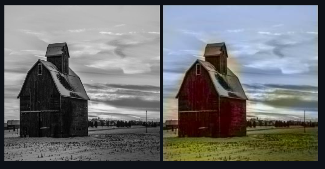
Output from my results
Conclusion
This is a very basic method of image colorization using autoencoders. There are many State-of-the-art models available now that yield better results but consider this a very basic step to learn about image colorization techniques.